Project Title: AEVCar Autonomous Vehicle

Project Overview

AEVCar is my autonomous vehicle project built around a ROS-based McMaster AEV / F1TENTH-style platform. The stack connects LiDAR, Intel RealSense depth sensing, BNO055 IMU feedback, VESC motor control, Ackermann steering, odometry, SLAM, collision assistance, and self-driving route planning.

• GitHub Repository: JustinLinKK/AEVCar

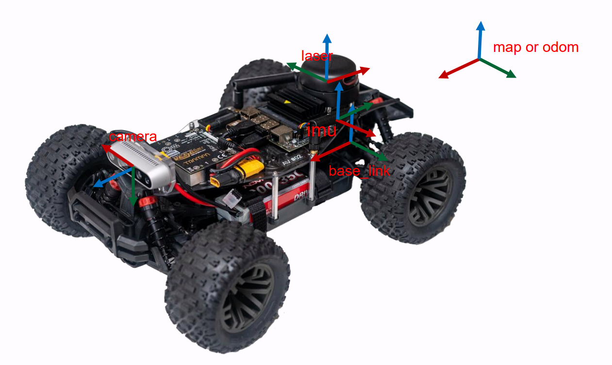
The project started from low-level ROS and vehicle bring-up, then grew into a full autonomy pipeline. I worked through motor telemetry, VESC command conversion, steering calibration, wheel odometry, IMU drift correction, LiDAR SLAM, obstacle avoidance, wall following, gap-based route planning, and depth-camera point-cloud fusion.

Objectives

• Vehicle Bring-Up: Build ROS nodes for joystick control, LiDAR testing, servo commands, VESC command publishing, and telemetry capture.
• Motor and Steering Integration: Convert high-level Ackermann commands into motor speed and steering servo commands, with rate-limited smoothing for safer actuation.
• IMU Drift Correction: Reduce heading drift from wheel-only odometry by using IMU yaw as a corrected orientation source.
• SLAM and Mapping: Use LiDAR scan matching with IMU-assisted transforms to build an occupancy-grid map of the environment.
• Obstacle Avoidance and Route Planning: Combine potential-field collision assistance, wall following, largest-gap selection, virtual separating barriers, and backup/turn recovery.
• Depth Fusion: Fuse RealSense depth-camera point clouds with LiDAR observations for a richer local planning representation.

Development Path

The project progressed through several layers, each one adding a missing piece of autonomy.

First, I set up the ROS environment on the Jetson Nano and connected the core packages: ackermann_msgs for drive commands, rplidar_ros for planar scan data, realsense2_camera for depth sensing, vesc_driver for motor control, and both rospy and roscpp nodes for Python/C++ development.

Then I built small nodes for manual vehicle control and data collection. The early scripts mapped joystick axes into duty-cycle and steering-servo commands, captured VESC state messages, converted raw logs into CSV files, and plotted motor speed, duty cycle, motor current, input current, and q-axis current. This gave me a practical view of how the PMSM/brushless motor responded before moving into higher-level autonomy.

After that, I integrated the real vehicle stack. The experiment launch path starts the VESC driver, RPLiDAR, BNO055 IMU, RealSense camera, mux controller, behavior controller, navigation node, collision-assistance node, and RViz. The simulator launch path keeps the same planning/control concepts but swaps in the simulated racecar, map server, simulated LiDAR, and simulated odometry.

• Simulation Path: simulator.launch starts a map server, racecar simulator, mux controller, behavior controller, random walker, keyboard control, navigation, collision assistance, and RViz.
• Real Vehicle Path: experiment.launch starts the VESC driver, RealSense camera, RPLiDAR, BNO055 IMU, static transforms, mux controller, behavior controller, navigation, collision assistance, and RViz.
• Vehicle Interface: experiment.cpp converts high-level velocity and steering commands into VESC motor RPM and servo position commands.
• Navigation: navigation.py and navigation_experiment.py process LiDAR/depth observations and publish AckermannDriveStamped commands.
• Safety and Control Selection: behavior_controller.cpp and mux.cpp switch between joystick, keyboard, navigation, collision assistance, random walking, and emergency braking.

Motor Driver and Actuation

The vehicle controller receives a standard ROS Ackermann command:

/drive -> speed in m/s + steering angle in radians

The physical vehicle cannot use that message directly. The experiment node translates it into the VESC command interface:

/commands/motor/speed
/commands/servo/position

For speed, the stack converts linear vehicle velocity into electrical RPM using the motor pole count, gear ratio, and wheel radius. The McMaster AEV parameters used in the lab material give a speed-to-ERPM gain of about 3182.12. For steering, the stack uses an affine calibration from desired steering angle to servo position:

servo_position = steering_gain * steering_angle + steering_offset

I also added command smoothing. Instead of jumping directly to the requested RPM or servo position, the experiment node clips each update by maximum acceleration and maximum steering velocity, then publishes smoothed commands at the configured driver smoother rate. This made the vehicle easier to test safely and reduced sudden actuation changes.

The next hardware-control step is deeper PMSM motor-driver integration. The current stack relies on the VESC abstraction for speed commands and telemetry, but the autonomy layer should eventually interface with a PMSM motor driver more directly, including command mapping, feedback ingestion, safety limits, and fault handling.

IMU Drift Correction

Wheel odometry alone accumulates angular error because steering angle, wheel slip, motor response, and calibration error compound over time. I implemented two odometry paths in experiment.cpp: one from the kinematic bicycle model and one corrected by IMU yaw.

The wheel-only path estimates vehicle speed from VESC feedback, derives steering angle from the servo command, and computes angular velocity with:

angular_velocity = speed * tan(steering_angle) / wheelbase

It then integrates x, y, and yaw over time. This works for short motion, but the heading can drift when the actual steering angle differs from the estimated steering angle.

The IMU-corrected path reads the BNO055 orientation quaternion, extracts roll, pitch, and yaw, and stores the first yaw measurement as the initial reference. After initialization, the vehicle still integrates position using measured speed, but it replaces the heading source with:

yaw_imu = imu_yaw - init_yaw

That produces a corrected /odom_imu estimate where position comes from vehicle speed integration and orientation follows the IMU heading. The result is more stable during turns, where small steering calibration errors can quickly make wheel-only odometry diverge.

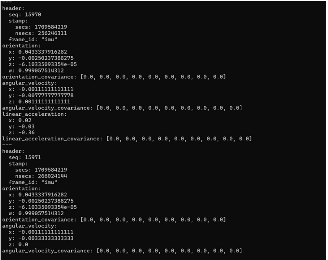
The project also includes an imu_tf_pkg node that subscribes to IMU data and publishes a TF transform from a stabilized reference frame to the vehicle frame. This gave the SLAM and visualization stack a consistent way to connect map, odom, base_link, imu, laser, and camera frames.

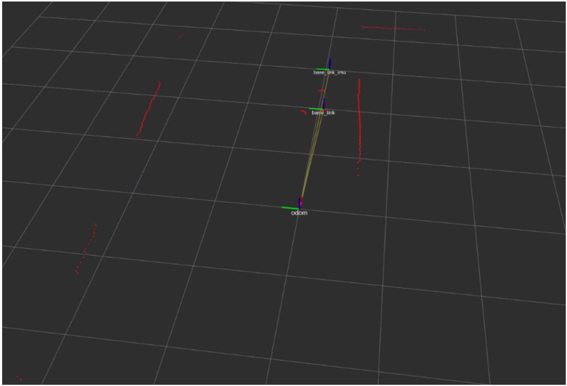
The IMU correction was not only a telemetry change; it changed how scan data lined up in RViz. With the IMU-assisted odometry frame, base_link_imu stays aligned to the vehicle's measured yaw instead of only following the integrated wheel model. That made LiDAR scan matching easier to interpret because scan endpoints, odometry, and the vehicle frame moved together more consistently.

LiDAR SLAM and Mapping

For mapping, I used Hector SLAM / scan matching with the RPLiDAR and IMU-assisted transforms. Hector SLAM builds an occupancy-grid map from LiDAR scans and aligns new scans against the map learned so far. It is useful for small robotic platforms because it can run online with relatively low compute cost.

The launch configuration sets up static transforms from base_link to the LiDAR, IMU, and camera frames. The LiDAR scan is corrected into the expected vehicle frame, and Hector mapping uses scan matching to estimate motion and update the occupancy grid. I configured mapping with a 0.05 m map resolution, multiple map resolution levels, and update thresholds for both distance and angle.

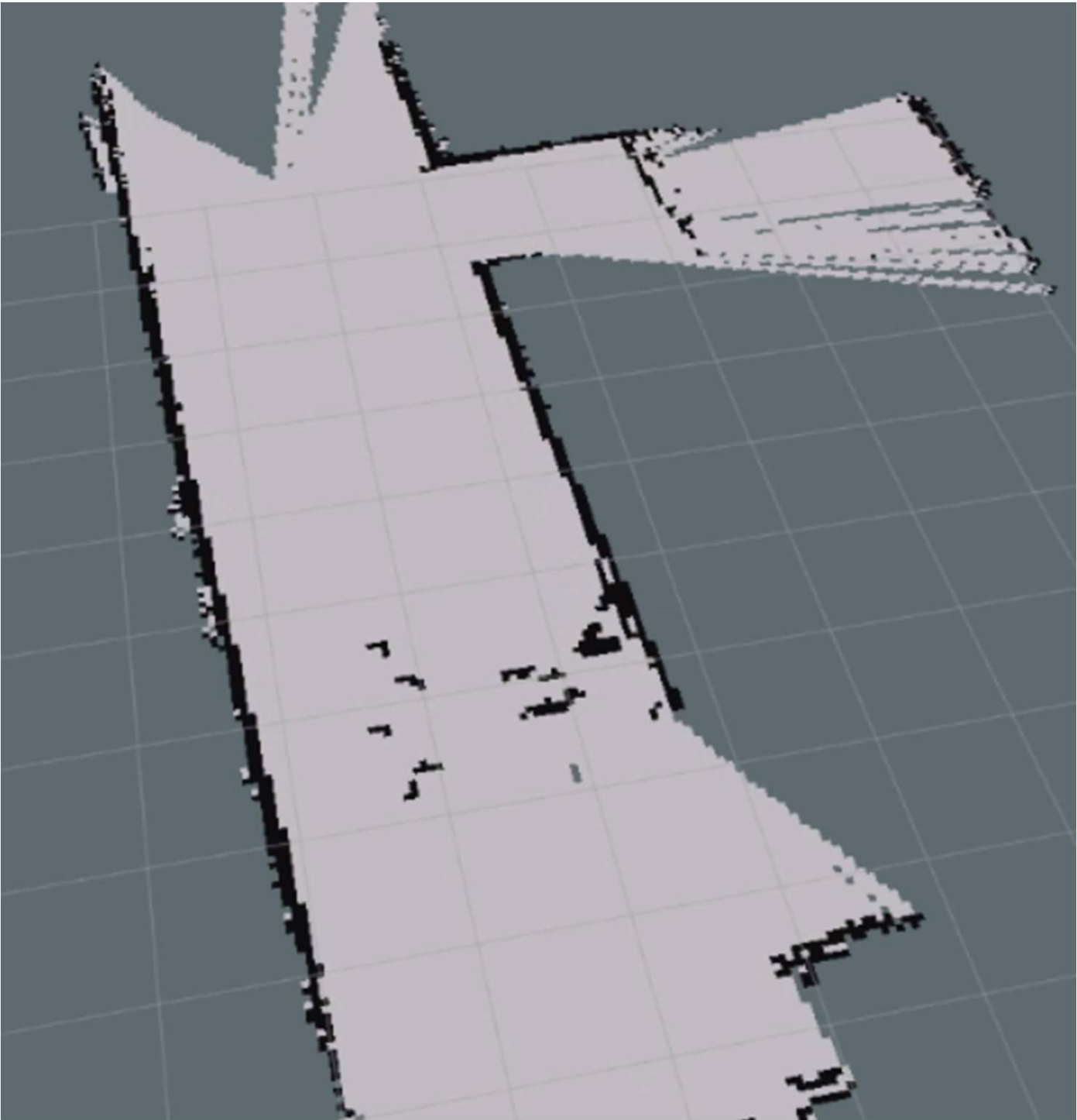
The Lab 7 report showed an important practical limitation: without IMU calibration, the scan matcher could still produce a map, but the scan angle and accumulated map quality were worse. With IMU-assisted orientation, the scan alignment was more consistent. Slowly driving the car produced a recognizable hallway map, especially in areas the car had already passed. Some blind-spot cones remained at certain angles until the car continued moving and scanned those regions from another viewpoint.

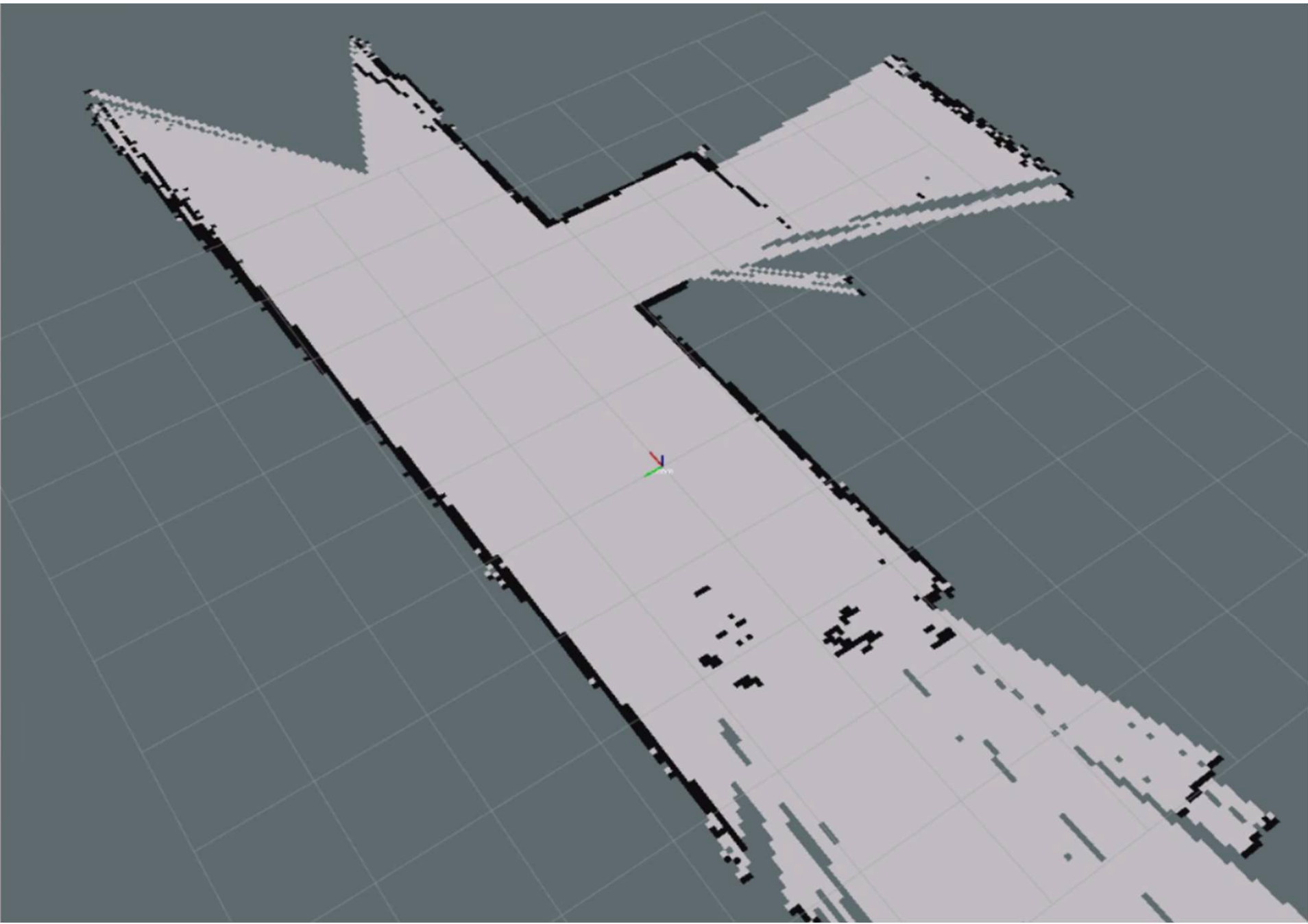
The map also showed deformation after turning the car around. This is a useful result because it exposes the difference between front-end scan matching and a full graph-SLAM pipeline: Hector SLAM can produce fast online occupancy maps, but this setup does not perform explicit loop closure to globally correct drift after revisiting an area.

LiDAR and Depth-Camera Fusion

The final navigation stack combines three complementary sensing inputs:

• RPLiDAR: A 2D scan used for obstacle detection, wall estimation, gap finding, and route following.
• RealSense Depth Camera: A forward depth point cloud used to detect objects that may be difficult to represent with a single planar LiDAR slice.
• IMU: A heading reference used to stabilize odometry and align motion estimates over time.

In navigation_experiment.py, the RealSense callback reads PointCloud2 data, removes invalid points, filters by distance and height, and converts the remaining points from the camera frame into the vehicle base_link frame. The transformed points are then projected into polar coordinates:

range = sqrt(x^2 + y^2)
angle = atan2(y, x)

The planner removes LiDAR returns inside the camera field of view, inserts the filtered camera points, and sorts the combined observation list by angle. This gave the route planner one fused local obstacle representation instead of two disconnected sensor streams.

Collision Assistance

Before full self-driving, I implemented a driver-assist collision avoidance layer. This node listens to joystick commands, odometry, and LiDAR scans, then publishes corrected Ackermann commands.

The algorithm looks only at the front 180-degree LiDAR field of view. It groups consecutive LiDAR beams below the obstacle-distance threshold into obstacle clusters, chooses the nearest point in each cluster, and computes a repulsive force from each obstacle. The force grows as the obstacle gets closer:

repulsive effect grows with (1 - obstacle_threshold / obstacle_distance)

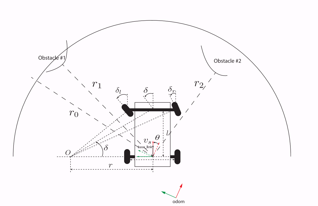
The x component of this correction reduces or modifies desired velocity, while the y component modifies the steering command. The final command blends user input with obstacle correction through tunable velocity and steering correction gains. This produced a safety layer that could assist manual driving without fully taking control away from the operator.

Obstacle Avoidance and Route Planning

The autonomous route planner evolved through two control methods.

The first method is wall following. It estimates left and right wall distances from selected LiDAR beams, computes the angle of each wall relative to the vehicle, and uses a feedback-linearizing PD controller to regulate wall distance. It can track the left wall, the right wall, or the difference between left and right wall distance. The steering command is computed from wall-distance error and wall-distance rate.

The second method improves on simple wall following by using largest-gap planning and virtual separating barriers.

1. LiDAR ranges in the forward field of view are preprocessed. Returns inside the safety distance are set to zero, and valid ranges are capped by the maximum LiDAR range.
2. The planner finds the longest consecutive sequence of nonzero returns, which represents the largest drivable gap.
3. The desired heading is computed as a range-weighted average of beam angles inside that gap.
4. The planner samples obstacle points to the left and right of the desired heading.
5. A quadratic program estimates virtual separating line barriers that keep the obstacle points outside the drivable corridor.
6. The steering controller centers the vehicle between the two virtual barriers using PD-style distance feedback.

The virtual-barrier method is more robust than using only two fixed wall beams because it can handle corners, non-flat walls, and obstacle shapes that do not look like clean corridor walls. The implementation supports both independent left/right barrier optimization and a parallel-barrier formulation inspired by support-vector-machine separation.

To avoid erratic steering, the barrier estimate is smoothed over time using an exponential update term:

alpha = 1 - exp(-dt / tau)

Velocity is also reduced when the front scan reports nearby obstacles:

velocity = nominal_velocity * (1 - exp(-max(front_distance - stop_distance, 0) / decay))

The route behavior also includes recovery states:

1. Normal: Follow the selected gap and wall estimate.
2. Backup: Reverse when the front path is blocked.
3. Turn: Rotate toward the direction with more free space before returning to normal navigation.

This makes the behavior more reliable in dead ends: the vehicle can stop, back up, choose the direction with the largest free-space score, turn, and then resume normal navigation.

Temporal Obstacles and Map Handling

The simulator and mapping stack distinguish between an original static map and a current working map. The simulator stores both original_map and current_map, supports inserting obstacles into the current occupancy grid, and includes a clear-obstacle path that restores the map back to the original baseline.

The design goal is to avoid treating every temporary object as permanent structure. A moved chair, person, or transient obstacle should affect immediate local planning, but it should not permanently corrupt the baseline map. In the project page I frame this as local map maintenance and working-map management rather than claiming a full production-grade obstacle-decay system.

Hardware and Software Stack

• Framework: ROS 1
• Compute: Jetson Nano / onboard ROS computer
• Vehicle Model: McMaster AEV / F1TENTH-style Ackermann platform
• Compute and Control: ROS nodes with C++ and Python
• Sensors: RPLiDAR, Intel RealSense depth camera, BNO055 IMU
• Actuation: VESC motor controller, PMSM/brushless traction motor, servo steering, and planned lower-level PMSM motor-driver integration
• Messages: LaserScan, PointCloud2, Imu, Odometry, AckermannDriveStamped
• Algorithms: IMU-yaw odometry correction, Hector SLAM, potential-field collision assistance, feedback-linearizing PD wall following, largest-gap planning, QP virtual barriers, backup/turn state machine
• Visualization: RViz TF frames, map server output, wall_markers, scan views, and occupancy-grid maps

Outcomes

• Built a ROS autonomous vehicle stack that connects simulation, sensor processing, odometry, planning, safety, and real actuation.
• Implemented Ackermann-to-VESC conversion with motor speed calibration, servo calibration, and smoothed command publishing.
• Captured and processed VESC telemetry for motor speed, duty cycle, motor current, input current, and q-axis current.
• Implemented wheel odometry and IMU-yaw-corrected odometry to reduce heading drift.
• Ran LiDAR-based Hector SLAM with IMU and TF integration to generate occupancy-grid maps.
• Implemented driver-assist obstacle avoidance using LiDAR obstacle clustering and potential-field correction.
• Implemented wall following and improved it with largest-gap selection, QP virtual barriers, and backup/turn recovery.
• Integrated RealSense depth point clouds with LiDAR scan data for a fused local planning representation.
• Identified the next hardware-control step: developing integration support for a PMSM motor driver so the autonomy stack can interface with a broader motor-control platform.

Why It Matters

This project mattered because it forced the autonomy problem into one integrated system. It was not only about detecting obstacles, or only about writing a controller. The vehicle needed motor calibration, sensor drivers, coordinate transforms, odometry correction, SLAM, map handling, local planning, steering control, safety modes, and real motor commands to agree with each other.

That is the part of robotics I find most interesting: every layer can work in isolation, but the real engineering challenge is making the full stack behave as one reliable system.