Project Title: DFT Signal Analysis and Tone Decoder

Project Overview

This project uses MATLAB, the discrete Fourier transform, and the fast Fourier transform to analyze audio signals in the frequency domain. The workflow starts with a clean tone signal, identifies its sinusoidal components, reconstructs the waveform from those measured components, and then applies the same spectral-analysis method to decode a noisy tone-symbol message.

The main idea was to move from time-domain listening and plotting into quantitative spectrum analysis. Once the FFT exposed which frequencies were present, the same approach could be reused as a simple receiver for a message encoded as combinations of sinusoidal tones.

Objectives

• Inspect Audio Waveforms: Read .wav signals in MATLAB and plot short time-domain windows for manual structure checks.
• Extract Frequency Content: Use fft, fftshift, and single-sided magnitude spectra to identify dominant sinusoidal components.
• Reconstruct a Source Signal: Generate a synthetic waveform from the measured frequencies and magnitudes.
• Decode Tone Symbols: Analyze 1-second windows of a noisy audio message and map active tones back to characters using a codebook.
• Build a Repeatable MATLAB Workflow: Keep the analysis broken into small scripts for waveform inspection, spectral plotting, synthesis, and symbol decoding.

Signal Analysis Workflow

The first signal, tones2022.wav, is a 10-second mono audio file sampled at 16 kHz. A 5 ms time-domain window shows a repeated waveform, but the component frequencies are much easier to identify after transforming the signal into the frequency domain.

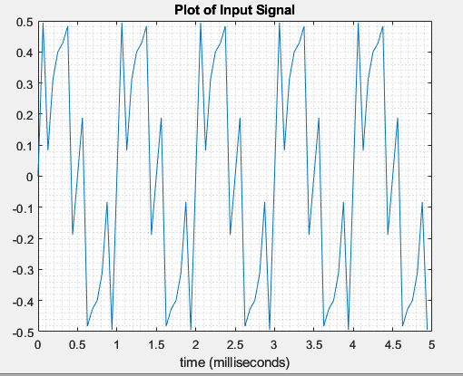
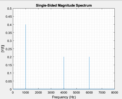
The single-sided magnitude spectrum isolated three dominant components:

Frequency	Magnitude
1000 Hz	0.4
4000 Hz	0.2
6000 Hz	0.2

Using those values, the tone signal was reconstructed as a sum of sinusoids. The reconstructed waveform matched the original time-domain plot, which validated the frequency-domain measurements.

MATLAB Implementation

The MATLAB scripts are organized by analysis task rather than as one large program:

• Waveform inspection: read the audio signal with audioread, build a time vector from the sample rate, and plot the first 5 ms.
• FFT / FFT-shift comparison: compute the DFT with fft, center the spectrum with fftshift, and compare the different frequency-axis views.
• Single-sided spectrum extraction: normalize the FFT output and plot the positive-frequency magnitude spectrum from 0 Hz to the 8 kHz Nyquist limit.
• Tone reconstruction: synthesize the measured 1000 Hz, 4000 Hz, and 6000 Hz components at the recovered magnitudes.
• Per-symbol decoding: segment the noisy message into 1-second windows, compute each window's spectrum, and identify the active tone set for that symbol period.

This kept the workflow easy to debug: the same spectral plot used for the clean tone signal became the diagnostic tool for each message window.

Results

The second signal, SecretMessage2022.wav, is a 76-second mono audio file sampled at 16 kHz. It contains a noisy transmission where each 1-second symbol period encodes one character as a combination of tones.

The message used frequencies from 1000 Hz through 7000 Hz. For each second-long window, the decoder inspected the single-sided magnitude spectrum, selected the tones that rose above the noise floor, and matched that tone combination to the codebook.

The recovered message was:

Never let the fear of striking out keep you from playing the game. Babe Ruth.

Lessons Learned

• Frequency-domain views reveal structure that time-domain plots hide: the tone signal looks dense in a short waveform plot, but the FFT makes the three sinusoidal components explicit.
• Windowing the problem makes noisy decoding manageable: analyzing the secret message one symbol period at a time avoids mixing characters together.
• Normalization and axis construction matter: using the correct sample rate, signal length, and single-sided scaling is what turns FFT output into meaningful frequency and magnitude estimates.
• Simple DSP can behave like a receiver: once each encoded character has a known tone signature, FFT peak detection is enough to recover the transmitted text.

Outcome

This project became a compact DSP receiver pipeline: read audio, transform it, identify spectral peaks, synthesize a measured waveform, and decode a message from noisy tone symbols. It reinforced the practical connection between MATLAB implementation details and the signal-processing theory behind the DFT.